Portfolio Risk Formula: A Step-by-Step Investor Guide
Learn the portfolio risk formula step by step: calculate variance, covariance, and standard deviation to manage risk and make smarter investment decisions.
Portfolio Risk Formula: A Step-by-Step Investor Guide

Portfolio risk is measured by the standard deviation of portfolio returns, calculated as σp = √(wᵀΣw), where w is the vector of asset weights and Σ is the variance-covariance matrix of asset returns. For a two-asset portfolio, the formula expands to:

σp² = w₁²σ₁² + w₂²σ₂² + 2w₁w₂σ₁σ₂ρ₁₂
The key components of any portfolio risk formula are:
- w₁, w₂ — the proportion of total capital allocated to each asset
- σ₁², σ₂² — the individual asset variances (squared standard deviations)
- σ₁, σ₂ — the individual asset standard deviations
- ρ₁₂ — the correlation coefficient between the two assets' returns
- Σ — the full covariance matrix for multi-asset portfolios
The critical insight here: portfolio risk is not a simple weighted average of individual asset risks. It reflects how assets move together, which means a well-constructed portfolio can carry less total risk than any single asset within it.
Table of Contents
- What portfolio risk actually means for your investments
- The exact formulas for two-asset and multi-asset portfolios
- How to calculate portfolio risk: a worked example
- How correlation shapes portfolio risk and diversification
- Related risk concepts and the limits of the formula
- How Evibe handles portfolio risk analysis for you
- Evibe puts your portfolio risk data in one place
- Key Takeaways
What portfolio risk actually means for your investments
Portfolio risk quantifies how much a portfolio's actual returns are likely to deviate from its expected return. Technically, it is the standard deviation (or variance) of the portfolio's return distribution. A higher standard deviation means wider swings, more uncertainty, and more exposure to outcomes you did not plan for.
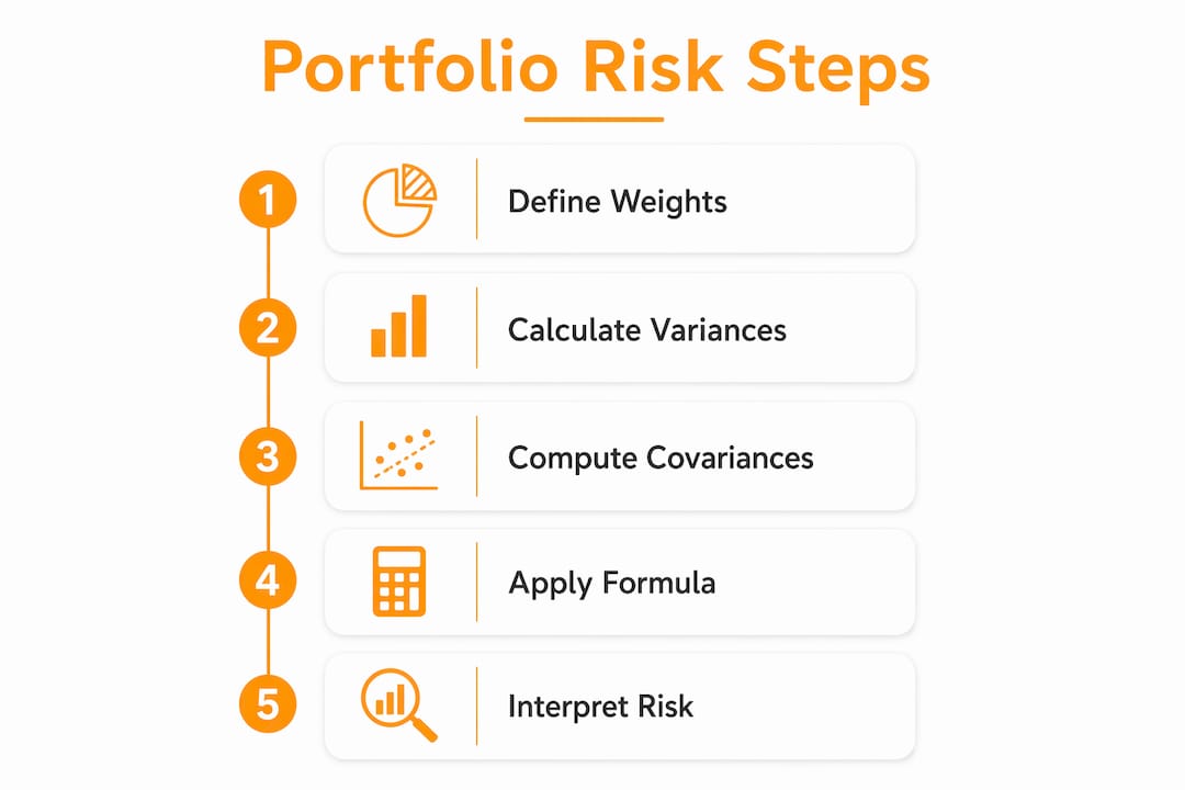
What makes portfolio risk distinct from individual asset risk is the interaction effect. Two assets, each with 20% annual volatility, do not necessarily produce a portfolio with 20% volatility. If those assets tend to move in opposite directions, the combined volatility can be substantially lower. This is the mathematical foundation of diversification.
Common portfolio risk management metrics include standard deviation, beta, Value-at-Risk (VaR), and Conditional Value-at-Risk (CVaR). Each serves a different purpose:
- Standard deviation — measures total return variability around the mean
- Beta — measures sensitivity to a benchmark (typically the S&P 500)
- VaR — estimates the maximum loss at a given confidence level over a set period
- CVaR — averages the losses that exceed the VaR threshold, capturing tail risk
Understanding portfolio risk matters because it directly shapes whether your portfolio can realistically achieve your financial goals within your tolerance for loss. A portfolio optimized only for return, with no attention to risk, is a portfolio waiting for a bad year to derail a long-term plan.
The exact formulas for two-asset and multi-asset portfolios
Two-asset portfolio variance
The two-asset portfolio variance formula is the clearest entry point into portfolio risk math:
σp² = w₁²σ₁² + w₂²σ₂² + 2w₁w₂σ₁σ₂ρ₁₂
Each variable has a precise financial meaning:
- w₁²σ₁² — the weighted variance contribution of Asset 1
- w₂²σ₂² — the weighted variance contribution of Asset 2
- 2w₁w₂σ₁σ₂ρ₁₂ — the interaction term, capturing how the two assets co-vary
- ρ₁₂ — ranges from −1 to +1; it is the correlation coefficient
- σ₁σ₂ρ₁₂ — this product equals the covariance between Asset 1 and Asset 2 (Cov₁₂)
Portfolio standard deviation is then: σp = √σp²
Multi-asset portfolio: matrix form
For portfolios with three or more assets, the formula generalizes using matrix algebra:
σp² = wᵀΣw
| Symbol | Meaning |
|---|---|
| w | Column vector of asset weights (must sum to 1) |
| wᵀ | Transpose of the weight vector (row vector) |
| Σ | Variance-covariance matrix (N × N for N assets) |
| σp² | Portfolio variance (scalar result) |
| σp | Portfolio standard deviation = √(wᵀΣw) |
The covariance matrix Σ has individual asset variances (σᵢ²) along its diagonal and pairwise covariances (Cov(i,j) = σᵢσⱼρᵢⱼ) in the off-diagonal positions. Every pair of assets contributes an interaction term, which is why adding assets to a portfolio changes risk in non-linear ways. As William Sharpe's portfolio theory framework demonstrates, portfolio variance is a quadratic function of portfolio composition, not a linear one — and that distinction is what makes quantitative analysis indispensable.
How to calculate portfolio risk: a worked example
Consider a two-asset portfolio with the following inputs:
| Parameter | Asset A (US Equity) | Asset B (US Bonds) |
|---|---|---|
| Weight | 0.60 (w₁) | 0.40 (w₂) |
| Annual Std Dev | 18% (σ₁) | 8% (σ₂) |
| Variance | 0.0324 (σ₁²) | 0.0064 (σ₂²) |
| Correlation (ρ₁₂) | 0.2 |
Step-by-step calculation:
A worked example shows how weighted variances and low positive correlation combine to reduce portfolio variance and risk below a simple weighted average of individual asset volatilities.

| Calculation Step | Value |
|---|---|
| Weighted variance, Asset A | 0.011664 |
| Weighted variance, Asset B | 0.001024 |
| Interaction term (2w₁w₂Cov) | 0.0027648 |
| Portfolio variance (σp²) | 0.0154528 |
| Portfolio risk (σp) | 12.43% |
Notice that a 60/40 weighted average of the individual standard deviations would give 0.60 × 18% + 0.40 × 8% = 14.0%. The actual portfolio risk of 11.86% is meaningfully lower, purely because of the low correlation between equities and bonds. That gap is diversification working in real numbers.
Pro Tip: When running these calculations yourself, always double-check that your weights sum to exactly 1.0. Even a small rounding error in weights compounds through the quadratic formula and distorts your final risk figure.
How correlation shapes portfolio risk and diversification
Correlation is the single most powerful lever in portfolio risk analysis. The correlation coefficient ρ ranges from −1 to +1, and where it sits determines how much risk reduction is achievable through combining assets.
- ρ = +1 (perfect positive correlation): The two assets move in lockstep. No diversification benefit exists. Portfolio risk equals the weighted average of individual risks.
- ρ = 0 (zero correlation): Assets move independently. Portfolio variance is reduced below the weighted average, since the interaction term contributes nothing.
- ρ = −1 (perfect negative correlation): Assets move in exactly opposite directions. In theory, a perfectly weighted combination can reduce portfolio risk to zero.
- ρ between 0 and +1 (most real-world pairs): Partial diversification benefit. The lower the correlation, the greater the risk reduction.
- ρ between −1 and 0: Strong diversification benefit; common in portfolios that combine equities with assets like Treasury bonds or gold during stress periods.
In practice, correlations between asset classes are rarely stable. Equities and bonds, historically low-correlation, have shown periods of positive correlation during inflationary environments. This is one reason why smart diversification requires ongoing monitoring rather than a set-it-and-forget-it approach.
Pro Tip: Do not rely on long-run average correlations alone. Correlations tend to spike toward +1 during market crises, precisely when you need diversification most. Building a portfolio that holds up under stressed correlations is a more resilient strategy than one optimized for calm-market conditions.
Related risk concepts and the limits of the formula
Variance vs. standard deviation vs. risk
These three terms are related but not interchangeable. Portfolio variance (σp²) is the raw mathematical output of the formula. Standard deviation (σp) is its square root and is expressed in the same units as returns (percentage), making it far more interpretable. When investors say "portfolio risk," they almost always mean standard deviation.
Key assumptions and where they break down
- Normal distribution of returns: The formula assumes asset returns follow a bell curve. In reality, return distributions have fat tails, meaning extreme losses occur more often than the model predicts.
- Stable covariance matrix: Historical covariances are used as proxies for future ones. During market dislocations, correlations shift sharply, and the covariance matrix becomes unreliable.
- Static weights: The formula calculates risk at a point in time. As prices move, actual portfolio weights drift, changing the risk profile continuously.
Beyond standard deviation: VaR, CVaR, and Sharpe ratio
Standard deviation treats upside and downside deviations equally, which is not how most investors experience risk. Three complementary metrics address this:
- Value-at-Risk (VaR): Estimates the maximum loss at a specified confidence level (e.g., 95%) over a defined period. Widely used but criticized for ignoring what happens beyond the threshold.
- CVaR (Conditional Value-at-Risk): Averages the losses that exceed the VaR cutoff, giving a more realistic picture of extreme tail risk. For portfolios with non-normal return distributions, CVaR is a superior complement to variance-based measures.
- Sharpe ratio: Divides excess return (above the risk-free rate) by standard deviation. It does not measure risk in isolation but tells you how much return you are earning per unit of risk taken.
None of these metrics replaces the portfolio risk formula. They work alongside it, each illuminating a different dimension of portfolio risk assessment that variance alone cannot capture.
How Evibe handles portfolio risk analysis for you
Running the portfolio risk formula manually is instructive, but doing it continuously across a real portfolio with dozens of positions across multiple asset classes is a different challenge. That is where Evibe is built to help.
Evibe consolidates stocks, ETFs, options, crypto, real estate, and other assets into a single dashboard, with automatic syncing from 1,000+ banks, brokerages and crypto exchanges across the US, Canada and Europe. Rather than maintaining spreadsheets and recalculating covariance matrices by hand, you get a live view of your entire net worth with risk metrics updated in real time.
Key features relevant to portfolio risk analysis:
- AI-driven risk and diversification analysis: Evibe's AI layer evaluates your portfolio's risk profile, flags concentration issues, and surfaces diversification gaps using easy-to-read metrics.
- Smart alerts: Get notified when market movements materially shift your portfolio's risk exposure, so you can act on changes rather than discover them after the fact.
- Benchmarking: Compare your portfolio's risk-adjusted performance against major indices to understand whether you are being compensated for the risk you are taking.
- Multi-asset coverage: From ETF-specific analytics and options Greeks to mark-to-market valuations on real estate and collectibles, Evibe captures the full picture.
- Glossary and educational resources: Evibe's built-in glossary helps you connect the terminology in this article directly to what you see in the app.
Pro Tip: Use Evibe's AI insights alongside the formulas in this article. When the app flags a high-risk concentration, run the two-asset formula manually for that pair to understand exactly which covariance term is driving the exposure. Theory and tooling together give you the clearest picture.
Evibe puts your portfolio risk data in one place

Calculating portfolio risk by hand is the right way to learn the formula. Managing it across a real, multi-asset portfolio is a different job, and that is what Evibe is built for. Instead of juggling spreadsheets and pulling correlation data from separate sources, you get a single dashboard that syncs your accounts automatically and applies AI-driven analysis to your actual holdings.
Evibe covers the full asset spectrum: stocks, ETFs, options, crypto, real estate, art, and more. The risk and diversification metrics update as markets move, so your portfolio risk picture stays current without manual recalculation. Smart alerts tell you when something material changes, and benchmarking shows you how your risk-adjusted returns compare to the indices that matter to you.
If you are serious about understanding and managing your portfolio's risk, the next step is straightforward: track your net worth with Evibe and let the AI analysis show you where your real exposures are.
Key Takeaways
The portfolio risk formula, σp = √(wᵀΣw), captures total portfolio uncertainty by combining asset weights, variances, and pairwise covariances, always producing a lower risk figure than a simple weighted average when correlations are below +1.
| Point | Details |
|---|---|
| Core formula | Portfolio risk is σp = √(wᵀΣw); for two assets, σp² = w₁²σ₁² + w₂²σ₂² + 2w₁w₂σ₁σ₂ρ₁₂. |
| Diversification math | A 60/40 equity-bond portfolio yields 12.43% risk, well below the 14.0% weighted average. |
| Correlation is the lever | Perfect positive correlation (ρ = +1) eliminates diversification; lower correlations reduce portfolio variance. |
| Formula limitations | Normal distribution and stable covariance assumptions break down in market stress; CVaR complements variance-based measures. |
| Evibe for live analysis | Evibe automates multi-asset risk tracking with AI-driven insights, smart alerts, and real-time benchmarking across all asset classes. |